

For weeks I was deep in linear algebra theory: matrices, determinants, eigenvalues, one practice set after another. Then a question started bothering me. What good is all this theory if I don't know what these transformations actually look like?
That question changed my plan. I put the practice problems down and set myself a new goal: build something that makes linear algebra visible. The result was an interactive geometric transformation visualiser. You type in a 2 × 2 matrix and watch what it does to a square, along with its determinant.
It taught me more than the problem sets had. Not just how matrices work, but how to think about them geometrically and algebraically at the same time. This post documents the whole journey: the questions I had, the insights, and the calculations I worked through by hand. All you need is basic familiarity with matrices and some curiosity about how they move space around.
Part 1: Why manual calculation still matters in the age of AI
Every calculation these days can be done by a calculator or an AI. Type in a matrix multiplication, press enter, and the answer appears instantly. So why do it by hand? Isn't that a waste of time?
Here's what I found: without manual calculation, you can't design mathematical algorithms. Let me explain why.

How your mind sees a calculation, and how a computer does
Say you multiply these two matrices by hand:
[ 2  1 ]   [ 1  0 ]
[ 0  3 ] × [ 0  1 ]
While you work, your mind is doing much more than arithmetic:
- You see the structure: rows of the first matrix meet columns of the second.
- You understand that each entry of the result is a dot product.
- You feel the relationship between input and output.
- You spot patterns: "the second matrix is the identity, so nothing changes. The answer is just the first matrix."
The computer sees a[0][0] * b[0][0] + a[0][1] * b[1][0] and executes it. Blind, mechanical steps, with no idea what is happening geometrically and no way to tell you why it matters.
It's faster, yes. But it's a calculator, not a mathematician.
Designing an algorithm needs intuition
When I sat down to design the engine for the visualiser, I had to answer three questions:
- How do I represent a shape mathematically?
- How do I apply a transformation to every point of that shape?
- How do I know whether the result is correct?
Every answer came from hours of multiplying matrices by hand. Because of that practice I knew that a shape is a collection of vertex vectors, that a transformation is matrix multiplication applied to each vertex, and that the determinant tells me what happened to area and orientation. Without it, I'd have been designing blind.
The paradox: you rarely need it, but you can't skip it

In real work you'll almost never multiply two 2 × 2 matrices by hand. But the boring practice of doing it is exactly what builds the mental models you need to architect a solution.
It's like cooking. You might use a food processor every day, but if you never learned to chop by hand you wouldn't understand how the angle of a cut changes the texture, why different vegetables need different techniques, or what a sharp blade does differently. Manual practice builds knowledge that lives in your intuition, not just your memory, and when you design algorithms, that intuition is everything.
The moment it clicked
My first plan for the algorithm was "multiply the matrix by the shape, done". But I didn't really understand why that worked until I pushed three points through a matrix by hand:
[ 0  -1 ] [ 1 ]   [ 0 ]
[ 1   0 ] [ 0 ] = [ 1 ]        (1, 0)  →  (0, 1)

[ 0  -1 ] [ 0 ]   [ -1 ]
[ 1   0 ] [ 1 ] = [  0 ]       (0, 1)  →  (-1, 0)

[ 0  -1 ] [ 1 ]   [ -1 ]
[ 1   0 ] [ 1 ] = [  1 ]       (1, 1)  →  (-1, 1)
Right goes to up, up goes to left, and the corner swings round with them. This matrix rotates every point 90° anticlockwise. Doing the calculation revealed the geometry hidden in the algebra.
Calculators give you answers. Manual calculation gives you understanding, and understanding is what lets you design algorithms that work.
Part 2: Representing a shape as a matrix

A shape in 2D is just a collection of points, and each point is a vector with an x and a y coordinate. The point (1, 0), for example, is the column vector:
v = [ 1 ]
    [ 0 ]
I wanted to visualise transformations of the unit square, whose four corners are (0, 0), (1, 0), (1, 1) and (0, 1). One small trick: to draw it as a closed outline, I repeat the starting point at the end, so the square is defined by five points.
I store all of them in a single 2 × 5 matrix, one vertex per column:
S = [ 0  1  1  0  0 ]   ← x-coordinates
    [ 0  0  1  1  0 ]   ← y-coordinates

      │  │  │  │  └── (0, 0)  back to the start
      │  │  │  └───── (0, 1)  top-left
      │  │  └──────── (1, 1)  top-right
      │  └─────────── (1, 0)  bottom-right
      └────────────── (0, 0)  start
Why columns and not rows?
This was one of my first questions. The answer is convention, but a convention that makes everything else clean.
We write a transformation as A · v: matrix on the left, vector on the right. For that product to work, v has to be a column:
[ a  b ] [ 1 ]   [ a·1 + b·0 ]   [ a ]
[ c  d ] [ 0 ] = [ c·1 + d·0 ] = [ c ]
If the point were a row, [1 0], you'd have to multiply from the other side, [1 0] × A, which gives [a b]: the first row of A rather than the first column. To get the right answer with rows, you would have to use the transpose of A everywhere. With columns, the natural formula A · v just works, and as we'll see, it lets you transform every vertex at once.
Part 3: A matrix is a transformation
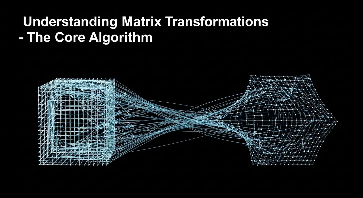
This is the core idea of linear algebra: a 2 × 2 matrix describes a transformation of 2D space. Rotation, scaling, shearing and reflection can all be written as a matrix.
So when someone types four numbers into the visualiser, they aren't just entering data. They're defining how space itself should bend.
The secret is in the columns. Space has two basic directions, the basis vectors î = (1, 0) pointing right and ĵ = (0, 1) pointing up, and the columns of the matrix say where each of them lands:
A = [ a  b ]     first column  (a, c) = where î lands
    [ c  d ]     second column (b, d) = where ĵ lands
Worked by hand: a 90° rotation
The 90° anticlockwise rotation matrix is:
A = [ 0  -1 ]
    [ 1   0 ]
Its columns say that î = (1, 0) lands on (0, 1), so right becomes up, and ĵ = (0, 1) lands on (−1, 0), so up becomes left. That's exactly a quarter turn. Let's confirm it on all four corners of the square:
(0, 0)  →  [ 0·0 + (-1)·0 ,  1·0 + 0·0 ]  =  ( 0, 0)
(1, 0)  →  [ 0·1 + (-1)·0 ,  1·1 + 0·0 ]  =  ( 0, 1)
(1, 1)  →  [ 0·1 + (-1)·1 ,  1·1 + 0·1 ]  =  (-1, 1)
(0, 1)  →  [ 0·0 + (-1)·1 ,  1·0 + 0·1 ]  =  (-1, 0)
The square has turned 90° anticlockwise. The corner that sat at the bottom right, (1, 0), now sits at the top, (0, 1).
The shortcut: one multiplication for every vertex
Here's the elegant part. Because S holds every vertex as a column, I don't need to transform them one at a time. A single matrix multiplication does all five at once:
                [ 0  -1 ]   [ 0  1  1  0  0 ]   [ 0  0  -1  -1  0 ]
S_transformed = [ 1   0 ] × [ 0  0  1  1  0 ] = [ 0  1   1   0  0 ]
Each column of the result is one transformed vertex, the same answers as above. That one line is the core algorithm of the whole project:
S_transformed = A × S_original
Part 4: The determinant is area scaling
With transformations working, I wanted to understand something deeper: what does a transformation do to area? The answer is a single number, the determinant. For a 2 × 2 matrix:
A = [ a  b ]
    [ c  d ]        det(A) = ad − bc
A simple formula, but what does it mean? It took many hand calculations before it sank in:
The determinant is the factor by which a transformation scales area. The unit square has area 1, so after the transformation its image has area |det(A)|.
Example 1: scaling
A = [ 2  0 ]
    [ 0  3 ]        det(A) = 2·3 − 0·0 = 6
The determinant predicts the area grows six-fold. Transforming the square:
[ 2  0 ]   [ 0  1  1  0  0 ]   [ 0  2  2  0  0 ]
[ 0  3 ] × [ 0  0  1  1  0 ] = [ 0  0  3  3  0 ]
The corners land on (0, 0), (2, 0), (2, 3) and (0, 3): a 2 × 3 rectangle with area 6. Exactly as predicted.
Example 2: a shear
H = [ 1  1 ]
    [ 0  1 ]        det(H) = 1·1 − 1·0 = 1
A determinant of 1 says the area shouldn't change. Let's check:
[ 1  1 ]   [ 0  1  1  0  0 ]   [ 0  1  2  1  0 ]
[ 0  1 ] × [ 0  0  1  1  0 ] = [ 0  0  1  1  0 ]
The corners land on (0, 0), (1, 0), (2, 1) and (1, 1): the square has been pushed sideways into a parallelogram. Its base is 1 and its height is 1, so its area is 1 × 1 = 1. The shape changed completely, but the area didn't, just as the determinant said.
Example 3: the sign matters
A = [ 1   0 ]
    [ 0  -1 ]       det(A) = 1·(−1) − 0·0 = −1
A negative determinant. Transforming the square:
[ 1   0 ]   [ 0  1  1  0  0 ]   [ 0  1   1   0  0 ]
[ 0  -1 ] × [ 0  0  1  1  0 ] = [ 0  0  -1  -1  0 ]
The square has been flipped across the x-axis: every point that was at y = 1 is now at y = −1. The area is still |−1| = 1, but the orientation has reversed, like a reflection in a mirror.
The strangest case: a determinant of zero
What if the determinant is exactly zero?
A = [ 1  1 ]
    [ 2  2 ]        det(A) = 1·2 − 1·2 = 0
Zero area. How can a square end up with no area at all?
[ 1  1 ]   [ 0  1  1  0  0 ]   [ 0  1  2  1  0 ]
[ 2  2 ] × [ 0  0  1  1  0 ] = [ 0  2  4  2  0 ]
The corners land on (0, 0), (1, 2), (2, 4) and (1, 2), and every one of them lies on the line y = 2x. The whole 2D square has been squashed onto a 1D line, and a line has no area. A matrix like this is called singular: it collapses space into a lower dimension, and that collapse can't be undone.
Putting the four cases together:
| Determinant | What happens to the square |
|---|---|
| det > 0 | Area scales by det; orientation is kept |
| det < 0 | Area scales by |det|; the shape is mirrored |
| det = 1 | Area is unchanged (rotations and shears) |
| det = 0 | The square collapses onto a line or a point |
Part 5: From theory to the engine
With the maths understood, the algorithm almost wrote itself:
- Input: four numbers a, b, c, d.
- Build the transformation matrix A from them.
- Define the unit square S as a 2 × 5 matrix.
- Transform it: S′ = A × S.
- Compute the determinant to report the area scaling.
No loops over vertices, no special cases. One matrix for the transformation, one for the shape, one multiplication, one determinant. Here's the heart of engine.py in my project:
# Create the transformation matrix
a = np.array([[x1, x2], [y1, y2]])

# Define the original square
b = np.array([[0, 1, 1, 0, 0], [0, 0, 1, 1, 0]])

# Apply the transformation
transformed_square = a @ b
The rest of the engine is presentation. Matplotlib draws the original square in green and the transformed shape in blue, puts the determinant in the title, and the image goes back to the browser through a small Flask endpoint.
A complete example
Let's run one input all the way through: a = 1, b = 0.5, c = 0, d = 1, a horizontal shear.
A = [ 1.0  0.5 ]
    [ 0.0  1.0 ]

[ 1.0  0.5 ]   [ 0  1  1  0  0 ]   [ 0.0  1.0  1.5  0.5  0.0 ]
[ 0.0  1.0 ] × [ 0  0  1  1  0 ] = [ 0.0  0.0  1.0  1.0  0.0 ]

det(A) = 1.0·1.0 − 0.5·0.0 = 1.0
The output corners are (0, 0), (1, 0), (1.5, 1) and (0.5, 1). The top edge has slid half a unit to the right, and the area is still 1.0. That's exactly what appears on screen.
Part 6: Experiments that taught me the most
Once the visualiser worked, I spent hours feeding it different matrices. These are the patterns that stuck.
Rotations never change area
Rotation by an angle θ has the form:
R(θ) = [ cos θ   −sin θ ]
       [ sin θ    cos θ ]
For 45°, cos 45° = sin 45° ≈ 0.707:
R(45°) = [ 0.707  -0.707 ]      det = 0.707·0.707 − (−0.707)·0.707 = 0.5 + 0.5 = 1
         [ 0.707   0.707 ]
Every rotation matrix has determinant 1, which makes sense: rotating something never changes its area or flips it. Checking one point, (1, 0) moves to (0.707, 0.707), exactly 45° anticlockwise.
Scaling: the determinant is width × height
A pure scaling matrix only has entries on its diagonal:
S = [ sx   0 ]       det(S) = sx · sy
    [  0  sy ]
With sx = 3 and sy = 2, the square becomes a 3 × 2 rectangle and det = 6. For a scaling matrix, the determinant formula is literally width × height.
Eigenvectors: the directions that don't turn
This one genuinely surprised me. I typed in:
A = [ 2  1 ]
    [ 1  2 ]
and noticed that the diagonal line y = x didn't rotate at all. It only stretched. Checking the point (1, 1) by hand:
[ 2  1 ] [ 1 ]   [ 3 ]       [ 1 ]
[ 1  2 ] [ 1 ] = [ 3 ] = 3 × [ 1 ]
The vector (1, 1) came out three times longer but pointing the same way. That makes it an eigenvector of A, and 3 is its eigenvalue:
A · v = λ · v with v = (1, 1), λ = 3
There's a second one hiding along y = −x: A · (1, −1) = (1, −1), an eigenvector with eigenvalue 1. Every other direction gets turned; these two only stretch. Watching that diagonal line simply grow while everything around it skewed and rotated taught me more about eigenvectors than any definition had.
Part 7: What changed in how I understand maths
Geometry makes algebra real. Matrices used to be grids of numbers. Now each one has a picture: numbers on the diagonal stretch along the axes, numbers off the diagonal shear, a negative determinant flips, and a zero determinant collapses a dimension. Algebra and geometry are two languages for the same thing.
The determinant is secretly simple. It's area scaling, nothing more. And ad − bc is exactly the area of the parallelogram whose sides are the matrix's columns, (a, c) and (b, d).
Manual calculation built the intuition. Every insight above came from working examples by hand. When I computed that the scaling matrix sends (1, 0) to (2, 0), I didn't just get an answer. I saw the x-coordinate double while y stayed put.
Simple algorithms can be powerful. The whole engine is output = matrix × shape. One line, and it handles every rotation, scaling, shear, reflection and combination of them. The power isn't in complicated code; it's in understanding the maths well enough to say it simply.
Conclusion
This project took me from abstract linear algebra to an intuition I can actually feel. The best way to understand a piece of maths isn't only to study it: it's to calculate it by hand, design an algorithm for it, and watch it move.
The tedious calculations on scrap paper turned out to be the most valuable part. They built the mental models that let me write a small, clean engine, and they revealed the geometry hiding inside the formulas. That same intuition is what later made SVD click for me, in the post on building a YouTube recommender.
The full code is on GitHub. Try a few matrices of your own, and see which one surprises you.